导航

这篇文章是 Transformer 完整版复现代码的深度解析。

本博客的 Transformer 系列文章共计四篇,导航如下:

前言

由哈佛的NLP组撰写的 The Annotated Transformer,用代码对应论文《Attention is all you need》的各个部分基本复现和还原了论文模型中初始版本的 Transformer,并给出了两个机器翻译的例子。而本文内容是在 The Annotated Transformer 的 Colab 版基础上,进一步精读 《Attention is all you need》中的 Transformer 结构和源码。作者之所以选择它进行解读,是因为它是一个单独的ipynb文件,如果我们要实际使用只需要全部执行单元格就行了。而一些比较大的库(比如Tensor2Tensor和OpenNMT等等)尽管也包含了Transformer的实现,但是对于理解论文和跑代码来说不够方便,为什么不选择更简单实用的现成品呢?

本文完整版及执行结果可见我在Google Colab的注释版副本 The Annotated Transformer by Harvard NLP .同时告诉大家一个小trick:不妨试着用Chatgpt进行代码讲解,本系列文章有相当一部分代码讲解都是经过Chatgpt辅助我理解消化的。读者可以尝试一下ChatGPT,我一般尊称它为 “Chat老师”,它是一个非常耐心的老师,(最重要的,它还是免费哒!)这让我想起了柏拉图或者孔夫子的教学方式——通过青年问禅师的对话体,来回答读者的困惑,并启发更深层次的哲学思考。

背景

The goal of reducing sequential computation also forms the foundation of the Extended Neural GPU, ByteNet and ConvS2S, all of which use convolutional neural networks as basic building block, computing hidden representations in parallel for all input and output positions. In these models, the number of operations required to relate signals from two arbitrary input or output positions grows in the distance between positions, linearly for ConvS2S and logarithmically for ByteNet. This makes it more difficult to learn dependencies between distant positions. In the Transformer this is reduced to a constant number of operations, albeit at the cost of reduced effective resolution due to averaging attention-weighted positions, an effect we counteract with Multi-Head Attention.

Self-attention, sometimes called intra-attention is an attention mechanism relating different positions of a single sequence in order to compute a representation of the sequence. Self-attention has been used successfully in a variety of tasks including reading comprehension, abstractive summarization, textual entailment and learning task-independent sentence representations. End-to-end memory networks are based on a recurrent attention mechanism instead of sequencealigned recurrence and have been shown to perform well on simple-language question answering and language modeling tasks.

To the best of our knowledge, however, the Transformer is the first transduction model relying entirely on self-attention to compute representations of its input and output without using sequence aligned RNNs or convolution.

翻译

减少序列计算(sequential computation)的目标也是Extended Neural GPU、ByteNet、以及ConvS2S等模型的基础,所有这些都是使用CNN作为基础块,对于所有的输入输出位置并行计算隐层表示。在这些模型当中,模型ConvS2S将任意输入输出信号联系起来要求操作的次数与这两者位置间的距离呈线性关系,而模型ByteNet则呈对数关系。 这使得学习远距离的依赖变得更加困难。然而在Transformer中,这个复杂度被减至一个常数操作,尽管由于平均 attention-weighted 位置在以减少有效地解析为代价,但我们提出一种 Multi-head Attention 用于抵消这种影响。

自我注意(self-attention),有时也称为内部注意,是一个注意力机制,这种注意力机制:将单个句子不同的位置联系起来,用于计算一个序列的表示。自我注意已经被成功应用在个各种各样的任务中,诸如阅读理解,抽象总结,文本蕴含,以及学习独立任务的句子表示中。端到端的记忆网络是基于递归注意力机制,而不是对齐序列递归,同时在单一语言问答系统以及语言建模任务中,端到端的网络已经被证明效果很好。

然而,据我们所知,Transformer 是第一个完全依赖于自我注意的推导模型。在接下来的部分中,我们将描述Transformer,自驱动的自我注意力机制,并且讨论它们的优缺点。

第一部分: 模型架构

Most competitive neural sequence transduction models have an encoder-decoder structure (cite). Here, the encoder maps an input sequence of symbol representations \((x_1, ..., x_n)\) to a sequence of continuous representations \(\mathbf{z} = (z_1, ..., z_n)\). Given \(\mathbf{z}\), the decoder then generates an output sequence \((y_1,...,y_m)\) of symbols one element at a time. At each step the model is auto-regressive (cite), consuming the previously generated symbols as additional input when generating the next.

翻译

大多数的神经序列推导模型有一个 encoder-decoder 结构。这里,encoder 将一个表示输入的字符序列 (\(x_1\),\(x_2\),...\(x_n\)) 映射成另一种连续表征序列 Z=(\(z_1\),\(z_2\),...\(z_m\))。 基于Z,decoder 每次产生一个元素 \(y_i\) 最终输出一个序列 Y=(\(y_1\),...\(y_m\)) 。Decoder中的每个步骤都是自回归的 —— 消耗之前产生的表征作为下次的输入。

在这里,"消耗 "意味着模型使用或吸收上一步生成的符号作为输入。换句话说,上一步生成的输出成为当前步骤的输入的一部分。

class EncoderDecoder(nn.Module):
"""
A standard Encoder-Decoder architecture.
Base for this and many other models.
"""
def __init__(self, encoder, decoder,
src_embed, tgt_embed, generator):
super(EncoderDecoder, self).__init__()
self.encoder = encoder
# Encoder对象
self.decoder = decoder
# Decoder对象
self.src_embed = src_embed
# 源语言序列的编码,包括词嵌入和位置编码
self.tgt_embed = tgt_embed
# 目标语言序列的编码,包括词嵌入和位置编码
self.generator = generator
# 生成器(Decoder后面 Linear + Softmax 部分)

def forward(self, src, tgt, src_mask, tgt_mask):
"Take in and process masked src and target sequences."
return self.decode(self.encode(src, src_mask), src_mask,
tgt, tgt_mask)
# 先对源语言序列进行编码,
# 结果作为memory传递给目标语言的编码器

def encode(self, src, src_mask):
# src = (batch.size, seq.length)
# src_mask 负责对src加掩码
return self.encoder(self.src_embed(src), src_mask)
# 对源语言序列进行编码,得到的结果为
# (batch.size, seq.length, 512)的tensor

def decode(self, memory, src_mask, tgt, tgt_mask):
return self.decoder(self.tgt_embed(tgt),
memory, src_mask, tgt_mask)
# 对目标语言序列进行编码,得到的结果为
# (batch.size, seq.length, 512)的tensor
class Generator(nn.Module):
"Define standard linear + softmax generation step."
def __init__(self, d_model, vocab):
# d_model=512, vocab = 目标语言词表大小
super(Generator, self).__init__()
self.proj = nn.Linear(d_model, vocab)
# 定义一个全连接层,可训练参数个数是(512 * trg_vocab_size) + trg_vocab_size

def forward(self, x):
return F.log_softmax(self.proj(x), dim=-1)
# x 类似于 (batch.size, sequence.length, 512)
# -> proj 全连接层 (30, 10, trg_vocab_size) = logits
# 对最后一个维度执行log_soft_max 得到(30, 10, trg_vocab_size)

The Transformer follows this overall architecture using stacked self-attention and point-wise, fully connected layers for both the encoder and decoder, shown in the left and right halves of Figure 1, respectively.

翻译

Transformer 遵循了这种总体的架构:在encoder和decoder中都使用数层self-attentionpoint-wise,全连接层。相对的各个部分正如Figure 1中左右两部分描述的一样。

Encoder and Decoder Stacks

Encoder

The encoder is composed of a stack of \(N=6\) identical layers.

翻译

Encoder 由6个相同的层叠加而成。

def clones(module, N):
"Produce N identical layers."
return nn.ModuleList([copy.deepcopy(module) for _ in range(N)])

关于 clones 函数

实现一个网络的深copy,也就是说copy一个新的对象,和原来的对象,完全分离,不分享任何存储空间,从而保证可训练参数,都有自己的取值或梯度。

比如可以用在copy N 个 EncoderLayer 组成 Encoder

class Encoder(nn.Module):
"Core encoder is a stack of N layers"
def __init__(self, layer, N):
# layer = one EncoderLayer object, N=6
super(Encoder, self).__init__()
self.layers = clones(layer, N)
# 深copy,N=6,
self.norm = LayerNorm(layer.size)
# 定义一个LayerNorm,layer.size=d_model=512
# 其中有两个可训练参数a_2和b_2

def forward(self, x, mask):
"Pass the input (and mask) through each layer in turn."
# x is alike (30, 10, 512)
# (batch.size, sequence.len, d_model)
# mask是类似于(batch.size, 10, 10)的矩阵
for layer in self.layers:
x = layer(x, mask)
# 进行6次EncoderLayer操作
return self.norm(x)
# 最后做一次LayerNorm,最后的输出也是(30, 10, 512)

Each layer has two sub-layers. The first is a multi-head self-attention mechanism, and the second is a simple, position-wise fully connected feed-forward network.

We employ a residual connection (cite) around each of the two sub-layers, followed by layer normalization (cite).

That is, the output of each sub-layer is \(\mathrm{LayerNorm}(x + \mathrm{Sublayer}(x))\), where \(\mathrm{Sublayer}(x)\) is the function implemented by the sub-layer itself. We apply dropout (cite) to the output of each sub-layer, before it is added to the sub-layer input and normalized.

To facilitate these residual connections, all sub-layers in the model, as well as the embedding layers, produce outputs of dimension \(d_{\text{model}}=512\).

翻译

Encoder 由6个相同的层叠加而成。每层又分成两个子层。第一层是multi-head self-attention机制,第二层则是简单的position-wise fully connected feed-forward network

在每个子层中,我们都使用残差网络,然后紧接着一个 layer normalization

也就是说:其实每个子层的实际输出是 LayerNorm(x+Sublayer(x)),其中Sublayer(x)是由sub-layer层实现的。

为了简化这个残差连接,模型中的所有子层都与 embedding 层相同,输出的结果维度都是 \(d_{model}\) = 512。

class LayerNorm(nn.Module):
"Construct a layernorm module (See citation for details)."
def __init__(self, features, eps=1e-6):
# features=d_model=512, eps=epsilon 用于分母的非0化平滑
super(LayerNorm, self).__init__()
self.a_2 = nn.Parameter(torch.ones(features))
# a_2 是一个可训练参数向量,(512)
self.b_2 = nn.Parameter(torch.zeros(features))
# b_2 也是一个可训练参数向量, (512)
self.eps = eps

def forward(self, x):
# x 的形状为(batch.size, sequence.len, 512)
mean = x.mean(-1, keepdim=True)
# 对x的最后一个维度,取平均值,得到tensor (batch.size, seq.len)
std = x.std(-1, keepdim=True)
# 对x的最后一个维度,取标准差,得(batch.size, seq.len)
return self.a_2 * (x - mean) / (std + self.eps) + self.b_2
# 本质上类似于(x-mean)/std,不过这里加入了两个可训练向量a_2 and b_2
# 以及分母上增加一个极小值epsilon,用来防止std为0的时候,除法溢出
class SublayerConnection(nn.Module):
"""
A residual connection followed by a layer norm.
Note for code simplicity the norm is first as opposed to last.
"""
def __init__(self, size, dropout):
# size=d_model=512; dropout=0.1
super(SublayerConnection, self).__init__()
self.norm = LayerNorm(size) # (512),用来定义a_2和b_2
self.dropout = nn.Dropout(dropout)

def forward(self, x, sublayer):
"Apply residual connection to any sublayer with the "
"same size."
# x is alike (batch.size, sequence.len, 512)
# sublayer是一个具体的MultiHeadAttention或者PositionwiseFeedForward对象

return x + self.dropout(sublayer(self.norm(x)))
# x (30, 10, 512) -> norm (LayerNorm) -> (30, 10, 512)
# -> sublayer (MultiHeadAttention or PositionwiseFeedForward)
# -> (30, 10, 512) -> dropout -> (30, 10, 512)

# 然后输入的x(没有走sublayer) + 和走sublayer后的结果,即实现了残差相加的功能
class EncoderLayer(nn.Module):
"Encoder is made up of self-attn and "
"feed forward (defined below)"
def __init__(self, size, self_attn, feed_forward, dropout):
# size = d_model = 512
# self_attn = MultiHeadAttention对象, first sublayer
# feed_forward = PositionwiseFeedForward对象,second sublayer
# dropout = 0.1 (e.g.)
super(EncoderLayer, self).__init__()
self.self_attn = self_attn
self.feed_forward = feed_forward
self.sublayer = clones(SublayerConnection(size, dropout), 2)
# 使用深度克隆方法,完整地复制出来两个SublayerConnection
self.size = size

def forward(self, x, mask):
"Follow Figure 1 (left) for connections."
# x shape = (30, 10, 512)
# mask 是(batch.size, 10,10)的矩阵,类似于当前一个词w,有哪些词是w可见的
# 源语言的序列的话,所有其他词都可见,除了"<blank>"这样的填充;
# 目标语言的序列的话,所有w的左边的词,都可见。
x = self.sublayer[0](x,
lambda x: self.self_attn(x, x, x, mask))
# lambda 匿名函数,说明见下文
# x (30, 10, 512) -> self_attn (MultiHeadAttention)
# shape is same (30, 10, 512) -> SublayerConnection -> (30, 10, 512)
return self.sublayer[1](x, self.feed_forward)
# x 和feed_forward对象一起,给第二个SublayerConnection

关于 SublayerConnection 实现和论文间的差异

论文中的执行顺序是 LayerNorm(x + Sublayer(x)),即把LayerNorm放残差和的外边了,对应的代码应该是return self.norm(x + self.dropout(sublayer(x)))。

这里的实现是先把x进行layernorm,然后扔给sublayer(例如multi-head self-attention, position-wise feed-forward),也有一定的道理(效果上并不差),类似于在复杂操作前,先layernorm。

关于 EncoderLayer 中,匿名函数 lambda 的说明

稍微难理解的是 EncoderLayer 的 forward 方法使用了lambda来定义一个匿名函数。这是因为之前我们定义的self_attn函数需要4个参数(Query的输入,Key的输入,Value的输入和Mask)。

因此这里我们使用lambda的技巧把它变成一个参数x的函数,mask可以看成已知的数。(lambda x 表示 lambda 的形参也叫 x),如果看到这里觉得难以理解的话,我们不妨把改写的函数抽离出来,记作 self_attn_lambda

def self_attn_lambda(x, mask):
return self.self_attn(x, x, x, mask)

def forward(self, x, mask):
x = self.sublayer[0](x, self_attn_lambda(x, mask))
return self.sublayer[1](x, self.feed_forward)

Decoder

The decoder is also composed of a stack of \(N=6\) identical layers.

In addition to the two sub-layers in each encoder layer, the decoder inserts a third sub-layer, which performs multi-head attention over the output of the encoder stack. Similar to the encoder, we employ residual connections around each of the sub-layers, followed by layer normalization.

We also modify the self-attention sub-layer in the decoder stack to prevent positions from attending to subsequent positions. This masking, combined with fact that the output embeddings are offset by one position, ensures that the predictions for position \(i\) can depend only on the known outputs at positions less than \(i\).

翻译

decoder 同样是由 N=6 个相同layer组成的栈。

除了encoder layer中的两个子层之外,decoder 还插入了第三个子层,这层的功能就是:利用 encoder 的输出,执行一个multi-head attention。与encoder相似,在每个子层中,我们都使用一个残差连接,接着在其后跟一个layer normalization。

为了防止当前位置看到后序的位置,我们同样修改了decoder 栈中的self-attention 子层。这个masking,是基于这样一种事实:输出embedding 偏移了一个位置,确保对位置i的预测仅仅依赖于位置小于i的、已知的输出。

class Decoder(nn.Module):
"Generic N layer decoder with masking."
def __init__(self, layer, N):
# layer = DecoderLayer object
# N = 6
super(Decoder, self).__init__()
self.layers = clones(layer, N)
# 深度copy 6次DecoderLayer
self.norm = LayerNorm(layer.size)
# 初始化1个LayerNorm

def forward(self, x, memory, src_mask, tgt_mask):
for layer in self.layers:
x = layer(x, memory, src_mask, tgt_mask)
# 执行6次DecoderLayer
return self.norm(x)
# 执行1次LayerNorm
class DecoderLayer(nn.Module):
"Decoder is made of self-attn, src-attn, "
"and feed forward (defined below)"
def __init__(self, size, self_attn, src_attn,
feed_forward, dropout):
# size = d_model=512,
# self_attn = one MultiHeadAttention object,目标语言序列的注意力层
# src_attn = second MultiHeadAttention object, 目标语言序列和源语言序列之间的注意力层
# feed_forward 全连接层
# dropout = 0.1
super(DecoderLayer, self).__init__()
self.size = size # 512
self.self_attn = self_attn
self.src_attn = src_attn
self.feed_forward = feed_forward
self.sublayer = clones(SublayerConnection(size, dropout), 3)
# 需要三个SublayerConnection, 分别在
# self.self_attn, self.src_attn 和 self.feed_forward 的后边

def forward(self, x, memory, src_mask, tgt_mask):
"Follow Figure 1 (right) for connections."
m = memory # (batch.size, sequence.len, 512)
# 来自源语言序列的Encoder之后的输出
# 作为memory供目标语言的序列检索匹配
x = self.sublayer[0](x,
lambda x: self.self_attn(x, x, x, tgt_mask))
# 通过一个匿名函数,来实现目标序列的自注意力编码
# 结果扔给sublayer[0]:SublayerConnection
x = self.sublayer[1](x,
lambda x: self.src_attn(x, m, m, src_mask))
# 通过第二个匿名函数,来实现目标序列和源序列的注意力计算
# 结果扔给sublayer[1]:SublayerConnection
return self.sublayer[2](x, self.feed_forward)
# 走一个全连接层,然后结果扔给sublayer[2]:SublayerConnection
def subsequent_mask(size):
"Mask out subsequent positions."
# e.g., size=10
attn_shape = (1, size, size) # (1, 10, 10)
subsequent_mask = np.triu(np.ones(attn_shape), k=1).astype('uint8')
# triu: 负责生成一个三角矩阵,k-th对角线以下都是设置为0
# 上三角中元素为1.

return torch.from_numpy(subsequent_mask) == 0
# 反转上面的triu得到的上三角矩阵,修改为下三角矩阵。

关于subsequent_mask的三角矩阵

subsequent_mask = np.triu(np.ones(attn_shape), k=1).astype('uint8')

这里的k=1表示1号对角线,不太容易理解:举例子如下:

Below the attention mask shows the position each tgt word (row) is allowed to look at (column). Words are blocked for attending to future words during training.

def example_mask():
LS_data = pd.concat(
[
pd.DataFrame(
{
"Subsequent Mask": subsequent_mask(20)[0][x, y].flatten(),
"Window": y,
"Masking": x,
}
)
for y in range(20)
for x in range(20)
]
)

return (
alt.Chart(LS_data)
.mark_rect()
.properties(height=250, width=250)
.encode(
alt.X("Window:O"),
alt.Y("Masking:O"),
alt.Color("Subsequent Mask:Q", scale=alt.Scale(scheme="viridis")),
)
.interactive()
)


show_example(example_mask)

Attention

An attention function can be described as mapping a query and a set of key-value pairs to an output, where the query, keys, values, and output are all vectors. The output is computed as a weighted sum of the values, where the weight assigned to each value is computed by a compatibility function of the query with the corresponding key.

We call our particular attention "Scaled Dot-Product Attention". The input consists of queries and keys of dimension \(d_k\), and values of dimension \(d_v\). We compute the dot products of the query with all keys, divide each by \(\sqrt{d_k}\), and apply a softmax function to obtain the weights on the values.

In practice, we compute the attention function on a set of queries simultaneously, packed together into a matrix \(Q\). The keys and values are also packed together into matrices \(K\) and \(V\). We compute the matrix of outputs as:

翻译

一个Attention function 可以被描述成一个“映射query和一系列key-value pair 到输出”,其中 query, keys, values, output 都是一个向量。 这些权值是由 querys 和 keys 通过相关函数计算出来的。 【注:原文中的query就是没有复数形式】

本文中使用的attention 被称作Scaled Dot-Product Attention。输入包含了 \(d_k\) 维的queries 和 keys,以及values 的维数是 \(d_v\)。 我们使用所有的values计算query的dot products,然后除以 \(\sqrt{d_k}\) ,再应用一个softmax函数去获得值的权重。【需要关注value在不同地方的含义。是key-value,还是计算得到的value?】

实际处理中,我们将同时计算一系列 query 的 attention,并将这些queries 写成矩阵Q的形式。同样,将 keys, values 同样打包成矩阵K和矩阵V。计算公式如下

\[ \mathrm{Attention}(Q, K, V) = \mathrm{softmax}(\frac{QK^T}{\sqrt{d_k}})V \]

def attention(query, key, value, mask=None, dropout=None): 
# query, key, value的形状类似于(30, 8, 10, 64), (30, 8, 11, 64),
# 30是batch.size,即当前batch中有多少一个序列;8=head.num,注意力头的个数;
# 10=目标序列中词的个数,11=源语言序列传过来的memory中,当前序列的词的个数,
# 64是每个词对应的向量表示。
# 类似于,这里假定query来自target language sequence;
# key和value都来自source language sequence.
"Compute 'Scaled Dot Product Attention'"

d_k = query.size(-1) # d_k = 64
scores = torch.matmul(query, key.transpose(-2, -1)) / math.sqrt(d_k)
# 先是(30, 8, 10, 64)和(30, 8, 64, 11)相乘,
#(注意是最后两个维度相乘)得到(30,8,10,11),
# 代表10个目标语言序列中每个词和11个源语言序列的分别的“亲密度”。
# 然后除以sqrt(d_k)=8,防止过大的亲密度。
# 这里的scores的shape是(30, 8, 10, 11)

if mask is not None:
scores = scores.masked_fill(mask == 0, -1e9)
# 使用mask,对已经计算好的scores,按照mask矩阵,填-1e9,
# 然后在下一步计算softmax的时候,被设置成-1e9的数对应的值~=0,被忽视

p_attn = F.softmax(scores, dim = -1)
# 对scores的最后一个维度执行softmax,得到的还是一个tensor, (30, 8, 10, 11)
if dropout is not None:
p_attn = dropout(p_attn) #执行一次dropout
return torch.matmul(p_attn, value), p_attn

# 返回的第一项,是(30,8,10,11)乘以 value=(30,8,11,64),得到的tensor是(30,8,10,64),
# 和query的最初的形状一样。另外,返回p_attn,形状为(30,8,10,11).
# 注意,这里返回p_attn主要是用来可视化显示多头注意力机制。

The two most commonly used attention functions are additive attention (cite), and dot-product (multiplicative) attention. Dot-product attention is identical to our algorithm, except for the scaling factor of \(\frac{1}{\sqrt{d_k}}\). Additive attention computes the compatibility function using a feed-forward network with a single hidden layer. While the two are similar in theoretical complexity, dot-product attention is much faster and more space-efficient in practice, since it can be implemented using highly optimized matrix multiplication code.

While for small values of \(d_k\) the two mechanisms perform similarly, additive attention outperforms dot product attention without scaling for larger values of \(d_k\) (cite). We suspect that for large values of \(d_k\), the dot products grow large in magnitude, pushing the softmax function into regions where it has extremely small gradients (To illustrate why the dot products get large, assume that the components of \(q\) and \(k\) are independent random variables with mean \(0\) and variance \(1\). Then their dot product, \(q \cdot k = \sum_{i=1}^{d_k} q_ik_i\), has mean \(0\) and variance \(d_k\).). To counteract this effect, we scale the dot products by \(\frac{1}{\sqrt{d_k}}\).

翻译

最常用的两个 attention 是 additive attentiondot-product(multiplicative) attention。除了使用放缩因子 \(\frac{1}{\sqrt{d_k}}\) 之外,本文中使用的算法与Dot-product attention算法完全一致。Additive attention 使用一个只有一层的前向反馈网络计算compatibility function。然而两者在理论复杂度上是相似的,实际上,dot-product attention更快些,且空间效率更高些,这是因为它可以使用高度优化的矩阵乘法代码来实现。

而对于\(d_k\)的较小值,这两种机制的表现相似,但加法注意力比(\(d_k\)值较大而没有缩放的)点积注意力更胜一筹。我们怀疑,对于大的\(d_k\)值,点积的量级会变大,导致softmax函数进入到了梯度极小的区域。

为了说明点积变大的原因。假设\(q\)\(k\)的组成部分是独立的随机变量的组成部分是独立的随机变量,其均值为 \(0\),方差为 \(1\)。 那么它们的点积, \(q \cdot k = \sum_{i=1}^{d_k} q_ik_i\),其均值为\(0\),方差为\(d_k\)

为了抵消这种影响,我们将点积的比例定为 \(\frac{1}{\sqrt{d_k}}\)

关于 dot-product attention 为什么要 scale \(\frac{1}{\sqrt{d_k}}\)

李沐老师在【Transformer论文逐段精读】中对这部分的解读摘录如下:

\(d_k\)不是很大的时候,除不除都没关系。但是当\(d_k\)很大的时候,也就是向量较长,内积可能非常大。当内积值较大时,差距也会较大。

而又因为softmax的操作趋向于让大的更大,小的更小,也就是置信的地方更接近1,不置信的地方更接近0,由此得到收敛,因此梯度会很小甚至梯度消失,导致模型会很快“跑不动”,失去了学习的作用。

Multi-head attention allows the model to jointly attend to information from different representation subspaces at different positions. With a single attention head, averaging inhibits this.

\[ \mathrm{MultiHead}(Q, K, V) = \mathrm{Concat}(\mathrm{head_1}, ..., \mathrm{head_h})W^O \\ \text{where}~\mathrm{head_i} = \mathrm{Attention}(QW^Q_i, KW^K_i, VW^V_i) \]

Where the projections are parameter matrices \(W^Q_i \in \mathbb{R}^{d_{\text{model}} \times d_k}\), \(W^K_i \in \mathbb{R}^{d_{\text{model}} \times d_k}\), \(W^V_i \in \mathbb{R}^{d_{\text{model}} \times d_v}\) and \(W^O \in \mathbb{R}^{hd_v \times d_{\text{model}}}\).

In this work we employ \(h=8\) parallel attention layers, or heads. For each of these we use \(d_k=d_v=d_{\text{model}}/h=64\). Due to the reduced dimension of each head, the total computational cost is similar to that of single-head attention with full dimensionality.

翻译

Multi-head attention 允许模型从不同位置的不同表示空间中联合利用信息。如果只是单头attention ,那么平均将会抑制这种状况。

\[ \mathrm{MultiHead}(Q, K, V) = \mathrm{Concat}(\mathrm{head_1}, ..., \mathrm{head_h})W^O \\ \text{where}~\mathrm{head_i} = \mathrm{Attention}(QW^Q_i, KW^K_i, VW^V_i) \]

在这个文本中,投影矩阵分别为 \(W^Q_i \in \mathbb{R}^{d_{\text{model}} \times d_k}\)\(W^K_i \in \mathbb{R}^{d_{\text{model}} \times d_k}\)\(W^V_i \in \mathbb{R}^{d_{\text{model}} \times d_v}\)\(W^O \in \mathbb{R}^{hd_v \times d_{\text{model}}}\),其中 \(d_{\text{model}}\) 表示模型的维度,\(d_k\)\(d_v\) 分别表示注意力机制中的查询、键和值向量的维度,\(h\) 表示注意力头的数量。

在本论文中,我们使用h = 8 个并行的注意力层,或者说注意力头。其中每一个注意力头,我们使用 \(d_k=d_v=d_{\text{model}}/h=64\)。由于减少了每个头的维度,总的计算损失与单个完全维度的attention 是相似的。

class MultiHeadedAttention(nn.Module): 
def __init__(self, h, d_model, dropout=0.1):
# h=8, d_model=512
"Take in model size and number of heads."
super(MultiHeadedAttention, self).__init__()
assert d_model % h == 0 # We assume d_v always equals d_k 512%8=0
self.d_k = d_model // h # d_k=512//8=64
self.h = h # h=8
self.linears = clones(nn.Linear(d_model, d_model), 4)
# 定义四个Linear networks, 每个的大小是(512, 512)的,
# 每个Linear network里面有两类可训练参数,Weights,
# 其大小为512*512,以及biases,其大小为d_model=512。

self.attn = None
self.dropout = nn.Dropout(p=dropout)

def forward(self, query, key, value, mask=None):
# 注意,输入query的形状类似于(30, 10, 512),
# key.size() ~ (30, 11, 512),
# 以及value.size() ~ (30, 11, 512)

if mask is not None: # Same mask applied to all h heads.
mask = mask.unsqueeze(1) # mask后续细细分解。
nbatches = query.size(0) #e.g., nbatches=30

# 1) Do all the linear projections in batch from
# d_model => h x d_k
query, key, value = [l(x).view(nbatches, -1, self.h, self.d_k)
.transpose(1, 2) for l, x in
zip(self.linears, (query, key, value))]
# 这里是形成Q、K、V矩阵的过程,也是前三个Linear Networks的具体应用,
# 例如query=(30, 10, 512) -> Linear network -> (30, 10, 512)
# -> view -> (30, 10, 8, 64) -> transpose(1,2) -> (30, 8, 10, 64)
# 对于key和value,也是类似的,从(30, 11, 512) -> (30, 8, 11, 64)。

# 2) Apply attention on all the projected vectors in batch.
x, self.attn = attention(query, key, value, mask=mask,
dropout=self.dropout)
# 调用上面定义好的attention函数,输出的x形状为(30, 8, 10, 64);
# attn的形状为(30, 8, 10=target.seq.len, 11=src.seq.len)

# 3) "Concat" using a view and apply a final linear.
x = x.transpose(1, 2).contiguous().view(nbatches, -1, self.h * self.d_k)
# x ~ (30, 8, 10, 64) -> transpose(1,2) ->
# (30, 10, 8, 64) -> contiguous() and view ->
# (30, 10, 8*64) = (30, 10, 512)
return self.linears[-1](x)
# 执行第四个Linear network,把(30, 10, 512)经过一次linear network,
# 得到(30, 10, 512).
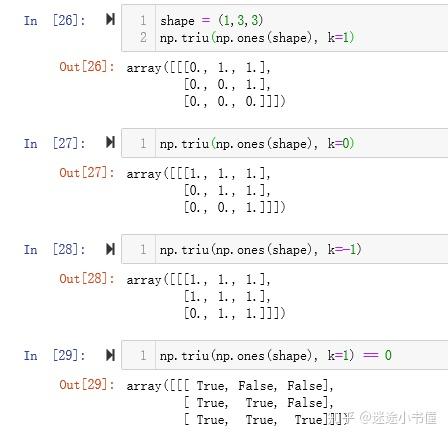
query, key, value = [l(x).view(nbatches, -1, self.h, self.d_k).transpose(1, 2) 
for l, x in zip(self.linears, (query, key, value))]

该代码的意思是将传入的Q、K、V三维矩阵经过一层全连接层后,重塑为四维矩阵,并且四维矩阵的第二、三维转置。torch.view函数的功能和numpy.reshape的功能差不多。下图可以很好的解释数据结构:

如图所示,最后得到的结果是个四维矩阵,维度依次是B、h、F、d_k。

  • B是Batch-size
  • h是多头自注意力机制中的头数
  • F是一个样本中的字符数,可以理解为一个句子中的单词个数
  • d_k是每个字符对应的embedding长度。

理解了这个类,Transformer的精髓也就理解得差不多了

Applications of Attention in our Model

The Transformer uses multi-head attention in three different ways: 1) In "encoder-decoder attention" layers, the queries come from the previous decoder layer, and the memory keys and values come from the output of the encoder. This allows every position in the decoder to attend over all positions in the input sequence. This mimics the typical encoder-decoder attention mechanisms in sequence-to-sequence models such as (cite).

  1. The encoder contains self-attention layers. In a self-attention layer all of the keys, values and queries come from the same place, in this case, the output of the previous layer in the encoder. Each position in the encoder can attend to all positions in the previous layer of the encoder.

  2. Similarly, self-attention layers in the decoder allow each position in the decoder to attend to all positions in the decoder up to and including that position. We need to prevent leftward information flow in the decoder to preserve the auto-regressive property. We implement this inside of scaled dot-product attention by masking out (setting to \(-\infty\)) all values in the input of the softmax which correspond to illegal connections.

Position-wise Feed-Forward Networks

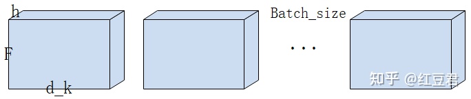
In addition to attention sub-layers, each of the layers in our encoder and decoder contains a fully connected feed-forward network, which is applied to each position separately and identically. This consists of two linear transformations with a ReLU activation in between.

\[\mathrm{FFN}(x)=\max(0, xW_1 + b_1) W_2 + b_2\]

While the linear transformations are the same across different positions, they use different parameters from layer to layer. Another way of describing this is as two convolutions with kernel size 1. The dimensionality of input and output is \(d_{\text{model}}=512\), and the inner-layer has dimensionality \(d_{ff}=2048\).

翻译

除了 attention sub-layers 【这里的attention sub-layers应该是一个名词】之外,encoder 和 decoder 的每层包含了一个全连接前馈网络,它分别相同地应用到每一个位置。这包含一个用ReLu做连接的两个线性转换操作。

\[\mathrm{FFN}(x)=\max(0, xW_1 + b_1) W_2 + b_2\]

尽管不同的位置有着相同的线性转换,但是它们使用不同的参数从一层到另一层。另一种描述这个的方法是:可以将这个看成是两个卷积核大小为1的卷积。输入和输出的维度都是 \(d_{\text{model}}=512\),同时,内部层维度是 \(d_{ff}=2048\)

class PositionwiseFeedForward(nn.Module):
"Implements FFN equation."
def __init__(self, d_model, d_ff, dropout=0.1):
# d_model = 512
# d_ff = 2048 = 512*4
super(PositionwiseFeedForward, self).__init__()
self.w_1 = nn.Linear(d_model, d_ff)
# 构建第一个全连接层,(512, 2048),其中有两种可训练参数:
# weights矩阵,(512, 2048),以及
# biases偏移向量, (2048)
self.w_2 = nn.Linear(d_ff, d_model)
# 构建第二个全连接层, (2048, 512),两种可训练参数:
# weights矩阵,(2048, 512),以及
# biases偏移向量, (512)
self.dropout = nn.Dropout(dropout)

def forward(self, x):
# x shape = (batch.size, sequence.len, 512)
# 例如, (30, 10, 512)
return self.w_2(self.dropout(F.relu(self.w_1(x))))
# x (30, 10, 512) -> self.w_1 -> (30, 10, 2048)
# -> relu -> (30, 10, 2048)
# -> dropout -> (30, 10, 2048)
# -> self.w_2 -> (30, 10, 512)是输出的shape

关于FFN的理解

实际上这就是一个MLP,但它是对每个词单独作用,并且保证对不同词作用的MLP参数相同。因此FFN实际就是一个线性层加上一个ReLU再加上一个线性层。
单隐藏层的 MLP,中间扩维到4倍 2048,最后投影回到 512 维度大小,便于残差连接。

Embeddings and Softmax

Similarly to other sequence transduction models, we use learned embeddings to convert the input tokens and output tokens to vectors of dimension \(d_{\text{model}}\). We also use the usual learned linear transformation and softmax function to convert the decoder output to predicted next-token probabilities. In our model, we share the same weight matrix between the two embedding layers and the pre-softmax linear transformation, similar to (cite). In the embedding layers, we multiply those weights by \(\sqrt{d_{\text{model}}}\).

翻译

与序列推导模型相似,我们使用embeddings 去将 input tokens和 output tokens转换成维度是 \({d_{model}}\) 的向量,我们同时使用通常学习的线性转换和softmax 函数,用于将decoder 输出转换成一个可预测的接下来单词的概率。在我们的模型中:在两个embedding layers 和 pre-softmax 线性转换中共用相同的权重矩阵。在embedding layers,我们将这些权重乘以\(\sqrt {d_{model}}\)

关于共享两个 Embedding 和 pre-softmax 权重矩阵

换句话说,同一组权重被用来将源语言和目标语言的词转换为连续矢量表示,以及将连续表示转换为目标语言词的预测。这种共享权重的做法有助于模型更有效地学习,因为它可以在源语言和目标语言中使用共同的模式。

共享权重是否有用,取决于源语言和目标语言之间的关系。如果这些语言有类似的结构和许多共同的词根,就像你提到的欧洲语系一样(本文用到了英法、英德翻译),那么共享权重就会有好处。然而,如果这些语言非常不同,就像中文和英文,那么共享权重可能没有用,甚至可能损害性能。

class Embeddings(nn.Module):
def __init__(self,d_model,vocab):
# d_model=512, vocab=当前语言的词表大小
super(Embeddings,self).__init__()
self.lut=nn.Embedding(vocab,d_model)
# one-hot转词嵌入,这里有一个待训练的矩阵lut,大小是vocab*d_model
self.d_model=d_model # 512
def forward(self,x):
# x ~ (batch.size, sequence.length, one-hot),
# one-hot大小=vocab,当前语言的词表大小

return self.lut(x)*math.sqrt(self.d_model)
# 输出的tensor大小类似于(batch.size, sequence.length, 512)
# 每个元素主动乘以sqrt(512)=22.6缩放比例

Embeddings类的forward函数中的math.sqrt(d_model)的乘法是一种归一化技术,用于缩放embedding。这个缩放系数用于确保两个embedding之间的点积与模型内的其他点积具有相似的大小,这有助于稳定训练过程,防止梯度变得过大或过小。

在实践中,比例因子的具体数值并不关键,不同的模型和实验中也使用了不同的数值。选择math.sqrt(d_model)作为比例因子是基于变换器的模型领域中常见的,它被用来确保嵌入中的值与模型的其他部分处于相似的尺度。然而,如果需要的话,你可以使用一个不同的比例系数,或者甚至完全不使用比例系数,这取决于你的具体使用情况和要求。

Positional Encoding

Since our model contains no recurrence and no convolution, in order for the model to make use of the order of the sequence, we must inject some information about the relative or absolute position of the tokens in the sequence. To this end, we add "positional encodings" to the input embeddings at the bottoms of the encoder and decoder stacks. The positional encodings have the same dimension \(d_{\text{model}}\) as the embeddings, so that the two can be summed. There are many choices of positional encodings, learned and fixed (cite).

In this work, we use sine and cosine functions of different frequencies:

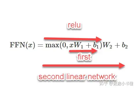
\[PE_{(pos,2i)} = \sin(pos / 10000^{2i/d_{\text{model}}})\]

\[PE_{(pos,2i+1)} = \cos(pos / 10000^{2i/d_{\text{model}}})\]

where \(pos\) is the position and \(i\) is the dimension. That is, each dimension of the positional encoding corresponds to a sinusoid. The wavelengths form a geometric progression from \(2\pi\) to \(10000 \cdot 2\pi\). We chose this function because we hypothesized it would allow the model to easily learn to attend by relative positions, since for any fixed offset \(k\), \(PE_{pos+k}\) can be represented as a linear function of \(PE_{pos}\).

In addition, we apply dropout to the sums of the embeddings and the positional encodings in both the encoder and decoder stacks. For the base model, we use a rate of \(P_{drop}=0.1\).

因为我们的模型没有包含RNN和CNN,为了让模型充分利用序列的顺序信息,我们必须获取一些信息关于tokens 在序列中相对或者绝对的位置。为了这个目的,我们在encoder 和 decoder 栈的底部 加上了positional encodings到 input embeddings中。这个positional embeddingembedding有相同的维度 \(d_{model}\)。有许多关于positional ecodings的选择。

在本论文中,我们使用不同频率的sine 和 cosine 函数。公式如下:
\[ \begin{aligned} PE_{pos,2i} = sin( \frac{pos}{10000^{2i/d_{model}}}) \\ PE_{pos,2i+1} = cos(\frac{pos}{10000^{2i/d_{model}}}) \end{aligned} \]

其中pos 是位置,i是维度。也就是说:每个位置编码的维度对应一个正弦曲线。波长形成了一个几何级数从2π 到 10000*2π。 选择这个函数的原因是:我们假设它让我们的模型容易学习到位置信息,因为对任何一个固定的偏移k, \(PE_{pos+k}\) 可以代表成一个 \(PE_{pos}\) 的线性函数。

class PositionalEncoding(nn.Module): 
"Implement the PE function."
def __init__(self, d_model, dropout, max_len=5000):
# d_model=512,dropout=0.1,
# max_len=5000,代表事先准备好长度为5000的序列的位置编码,其实没必要,一般100或者200足够了。
super(PositionalEncoding, self).__init__()
self.dropout = nn.Dropout(p=dropout)

# Compute the positional encodings once in log space.
pe = torch.zeros(max_len, d_model)
# (5000,512)矩阵,保持每个位置的位置编码,一共5000个位置,
# 每个位置用一个512维度向量来表示其位置编码
position = torch.arange(0, max_len).unsqueeze(1)
# (5000) -> (5000,1)
div_term = torch.exp(torch.arange(0, d_model, 2) *
-(math.log(10000.0) / d_model))
# (0,2,…, 4998)一共准备2500个值,供sin, cos调用
# 公式做了变形,详见下方说明
pe[:, 0::2] = torch.sin(position * div_term) # 偶数下标的位置
pe[:, 1::2] = torch.cos(position * div_term) # 奇数下标的位置
pe = pe.unsqueeze(0)
# (5000, 512) -> (1, 5000, 512) 为batch.size留出位置
self.register_buffer('pe', pe)
# The pe tensor is then registered as a buffer,
# which means it will not be part of the model's parameters
# and will not require gradients during the backward pass.

def forward(self, x):
x = x + Variable(self.pe[:, :x.size(1)], requires_grad=False)
# 接受 Embeddings 的词嵌入结果x,然后把自己的位置编码pe缩放成x.size(1)的长度,(封装成torch的Variable),加上去
# 由于self.pe[:, :x.size(1)]不是一个可学习的参数,所以设置requires_grad=False,表示不需要梯度。
# 例如,假设x是(30,10,512)的一个tensor,30是batch.size, 10是该batch的序列长度, 512是每个词的词嵌入向量;
# 则该行代码的第二项是(1, min(10, 5000), 512)=(1,10,512),
# 在具体相加的时候,会扩展(1,10,512)为(30,10,512),保证一个batch中的30个序列,都使用(叠加)一样的位置编码。
return self.dropout(x) # 增加一次dropout操作
# 注意,位置编码不会更新,是写死的,所以这个class里面没有可训练的参数。

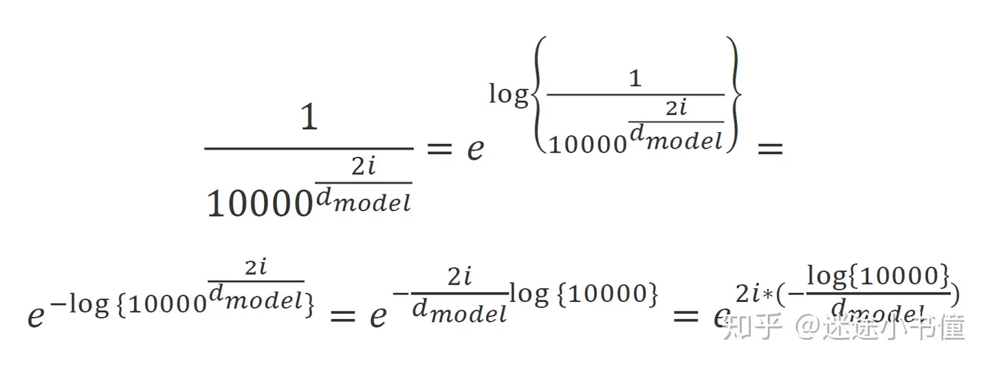
为了计算这个公式,上面的公式做了一系列变形,因此代码可能第一眼看上去和公式不像,下面以\(2i\)(偶数情况)为例子说明:

注意,位置编码不会更新,是写死的,所以这个class里面没有可训练的参数。

有了 EmbeddingsPositionalEncoding

在具体使用的时候,是通过torch.nn.Sequential来把他们两个串起来的:

# in Full Model
# nn.Sequential(Embeddings(d_model, src_vocab), c(position)),
# nn.Sequential(Embeddings(d_model, tgt_vocab), c(position))

Below the positional encoding will add in a sine wave based on position. The frequency and offset of the wave is different for each dimension.

关于位置编码的可视化

下面的位置编码将添加一个基于位置的正弦波。波的频率和偏移对于每个维度都是不同的。(最多)

def example_positional():
pe = PositionalEncoding(20, 0)
# d_model=20, dropout=0,max_len=5000
y = pe.forward(torch.zeros(1, 100, 20))
# x是(1, 100, 20)的一个tensor,1是batch.size, 100是该batch的序列长度, 20是每个词的词嵌入向量d_model;
# y (1, 100, 20),从d_model中选取dim
data = pd.concat(
[
pd.DataFrame(
{
"embedding": y[0, :, dim],
"dimension": dim,
"position": list(range(100)),
}
)
for dim in [4, 5, 6, 7]
]
)

return (
alt.Chart(data)
.mark_line()
.properties(width=800)
.encode(x="position", y="embedding", color="dimension:N")
.interactive()
)


show_example(example_positional)

We also experimented with using learned positional embeddings (cite) instead, and found that the two versions produced nearly identical results. We chose the sinusoidal version because it may allow the model to extrapolate to sequence lengths longer than the ones encountered during training.

翻译

我们还尝试使用学习到的位置嵌入(另一种方式得到的positional embeddding)来代替,发现这两个版本产生了几乎相同的结果。我们选择正弦版本是因为它可以让模型推断出比训练期间遇到的序列长度更长的序列长度。

关于positional embedding

位置嵌入是一个符号在序列中的位置的连续表示。它们被添加到符号的连续表示中(即词嵌入),以告知模型每个符号在输入序列中的相对或绝对位置。

有两种方法可以产生位置嵌入:学习型和正弦型。学习型位置嵌入是由神经网络生成的,并与模型的其他部分一起训练。正弦位置嵌入是使用一个数学函数生成的,如正弦或余弦,它将序列中的每个位置映射到一个独特的连续表示。

该论文的作者发现,这两个版本的位置嵌入在他们的实验中产生了几乎相同的结果。然而,他们选择了正弦波版本,因为它可能允许模型推断出比训练期间遇到的序列长度更长的序列。这是因为正弦函数是周期性的,可以无限期地重复模式,而学习的位置嵌入是由一个固定大小的神经网络产生的,可能不能很好地推广到更长的序列。

Full Model

Here we define a function from hyperparameters to a full model.

def make_model(src_vocab, tgt_vocab, N=6, 
d_model=512, d_ff=2048, h=8, dropout=0.1):
"Helper: Construct a model from hyperparameters."
# src_vocab = 源语言词表大小
# tgt_vocab = 目标语言词表大小

c = copy.deepcopy # 对象的深度copy/clone
attn = MultiHeadedAttention(h, d_model) # 8, 512
# 构造一个MultiHeadAttention对象

ff = PositionwiseFeedForward(d_model, d_ff, dropout)
# 512, 2048, 0.1
# 构造一个feed forward对象

position = PositionalEncoding(d_model, dropout)
# 位置编码

model = EncoderDecoder(
Encoder(EncoderLayer(d_model, c(attn), c(ff), dropout), N),
Decoder(DecoderLayer(d_model, c(attn), c(attn),
c(ff), dropout), N),
nn.Sequential(Embeddings(d_model, src_vocab), c(position)),
nn.Sequential(Embeddings(d_model, tgt_vocab), c(position)),
Generator(d_model, tgt_vocab))

# This was important from their code.
# Initialize parameters with Glorot / fan_avg.
for p in model.parameters():
if p.dim() > 1:
nn.init.xavier_uniform(p)
return model # EncoderDecoder 对象

关于参数初始化

for p in model.parameters():
if p.dim() > 1:
nn.init.xavier_uniform(p)

这段代码的作用是初始化Transformer模型的参数。"Glorot / fan_avg"是一种常用的初始化方法,也被称为"Xavier initialization"。该方法的目的是使得模型的参数有合适的初始值,以避免梯度消失和爆炸的问题。

因此,这段代码的重要性在于它为Transformer模型的学习提供了合适的初始条件,从而提高模型的学习效率和精度。在机器学习领域,初始参数的选择对于模型的效果有很大影响,因此该代码是很重要的。

Inference:

Here we make a forward step to generate a prediction of the model. We try to use our transformer to memorize the input. As you will see the output is randomly generated due to the fact that the model is not trained yet. In the next tutorial we will build the training function and try to train our model to memorize the numbers from 1 to 10.

在这里,我们向前迈出一步以生成模型的预测。我们尝试使用我们的转换器来记住输入。正如您将看到的那样,由于模型尚未训练,输出是随机生成的。在下一个教程中,我们将构建训练函数并尝试训练我们的模型来记住从 1 到 10 的数字。

def inference_test():
test_model = make_model(11, 11, 2)
test_model.eval()
src = torch.LongTensor([[1, 2, 3, 4, 5, 6, 7, 8, 9, 10]])
src_mask = torch.ones(1, 1, 10)

memory = test_model.encode(src, src_mask)
ys = torch.zeros(1, 1).type_as(src)

for i in range(9):
out = test_model.decode(
memory, src_mask, ys, subsequent_mask(ys.size(1)).type_as(src.data)
)
prob = test_model.generator(out[:, -1])
_, next_word = torch.max(prob, dim=1)
next_word = next_word.data[0]
ys = torch.cat(
[ys, torch.empty(1, 1).type_as(src.data).fill_(next_word)], dim=1
)

print("Example Untrained Model Prediction:", ys)


def run_tests():
for _ in range(10):
inference_test()


show_example(run_tests)

第二部分: 模型训练

训练

This section describes the training regime (训练机制) for our models.

We stop for a quick interlude to introduce some of the tools needed to train a standard encoder decoder model. First we define a batch object that holds the src and target sentences for training, as well as constructing the masks.

我们暂时停下来介绍一些训练标准编码器解码器模型所需的工具。首先,我们定义一个批处理对象,其中包含用于训练的 src 和目标句子,以及构建掩码。

Batches and Masking

class Batch:
"Object for holding a batch of data with mask during training."
def __init__(self, src, trg=None, pad=0):
# src: 源语言序列,(batch.size, src.seq.len)
# 二维tensor,第一维度是batch.size;第二个维度是源语言句子的长度
# 例如:[ [2,1,3,4], [2,3,1,4] ]这样的二行四列的,
# 1-4代表每个单词word的id

# trg: 目标语言序列,默认为空,其shape和src类似
# (batch.size, trg.seq.len),
# 二维tensor,第一维度是batch.size;第二个维度是目标语言句子的长度
# 例如trg=[ [2,1,3,4], [2,3,1,4] ] for a "copy network"
# (输出序列和输入序列完全相同)

# pad: 源语言和目标语言统一使用的 位置填充符号,'<blank>'
# 所对应的id,这里默认为0
# 例如,如果一个source sequence,长度不到4,则在右边补0
# [1,2] -> [1,2,0,0]

self.src = src
self.src_mask = (src != pad).unsqueeze(-2)
# src = (batch.size, seq.len) -> != pad ->
# (batch.size, seq.len) -> usnqueeze ->
# (batch.size, 1, seq.len) 相当于在倒数第二个维度扩展
# e.g., src=[ [2,1,3,4], [2,3,1,4] ]对应的是
# src_mask=[ [[1,1,1,1], [1,1,1,1]] ]
if trg is not None:
self.trg = trg[:, :-1] # 重要
# trg 相当于目标序列的前N-1个单词的序列
#(去掉了最后一个词)
self.trg_y = trg[:, 1:]
# trg_y 相当于目标序列的后N-1个单词的序列
# (去掉了第一个词<start>)
# 目的是(src + trg) 来预测出(trg_y),
# 这个在illustrated transformer中详细图示过。
self.trg_mask = \
self.make_std_mask(self.trg, pad)
self.ntokens = (self.trg_y != pad).data.sum()

@staticmethod
def make_std_mask(tgt, pad):
"Create a mask to hide padding and future words."
# 这里的tgt类似于:
# [ [2,1,3], [2,3,1] ] (最初的输入目标序列,分别去掉了最后一个词
# pad=0, '<blank>'的id编号
tgt_mask = (tgt != pad).unsqueeze(-2)
# 得到的tgt_mask类似于
# tgt_mask = tensor([[[1, 1, 1]],[[1, 1, 1]]], dtype=torch.uint8)
# shape=(2,1,3)
tgt_mask = tgt_mask & Variable(
subsequent_mask(tgt.size(-1)).type_as(tgt_mask.data))
# 先看subsequent_mask, 其输入的是tgt.size(-1)=3
# 这个函数的输出为= tensor([[[1, 0, 0],
# [1, 1, 0],
# [1, 1, 1]]], dtype=torch.uint8)
# type_as 把这个tensor转成tgt_mask.data的type(也是torch.uint8)

# 这样的话,&的两边的tensor.shape分别是(2,1,3), (1,3,3);
# tgt_mask = tensor([[[1, 1, 1]],[[1, 1, 1]]], dtype=torch.uint8)
# and
# tensor([[[1, 0, 0], [1, 1, 0], [1, 1, 1]]], dtype=torch.uint8)

# (2,3,3)就是得到的tensor
# tgt_mask.data = tensor(
# [[1, 0, 0],
# [1, 1, 0],
# [1, 1, 1]]], dtype=torch.uint8)
return tgt_mask

关于"Batch"类

用于存储和处理训练数据

__init__方法初始化了Batch对象的各个成员变量:

  • src:源语言序列
  • src_mask:源语言序列的掩码,用于表示序列中的某些位置是否有效
  • trg:目标语言序列(可选)
  • trg_y:目标语言序列的标签,即目标语言序列的下一个词
  • trg_mask:目标语言序列的掩码,表示该序列中哪些位置是有效的,用于注意力机制
  • ntokens:表示目标语言序列中有效词的数量

make_std_mask是一个静态方法,用于创建目标语言序列的mask。该方法的作用是防止注意力机制关注未来的预测词。它创建了一个mask,通过将目标语言序列中有效位置与subsequent_mask进行位运算来实现该目的。

Next we create a generic training and scoring function to keep track of loss. We pass in a generic loss compute function that also handles parameter updates.

接下来我们创建一个通用的训练和评分函数来跟踪损失。我们传入了一个通用的损失计算函数,该函数也处理参数更新。

Training Loop

class TrainState:
"""Track number of steps, examples, and tokens processed"""

step: int = 0 # Steps in the current epoch
accum_step: int = 0 # Number of gradient accumulation steps
samples: int = 0 # total # of examples used
tokens: int = 0 # total # of tokens processed
def run_epoch(
data_iter,
model,
loss_compute,
optimizer,
scheduler,
mode="train",
accum_iter=1,
train_state=TrainState(),
):
"""Train a single epoch"""
start = time.time()
total_tokens = 0
total_loss = 0
tokens = 0
n_accum = 0
for i, batch in enumerate(data_iter):
out = model.forward(
batch.src, batch.tgt, batch.src_mask, batch.tgt_mask
)
loss, loss_node = loss_compute(out, batch.tgt_y, batch.ntokens)
# loss_node = loss_node / accum_iter
if mode == "train" or mode == "train+log":
loss_node.backward()
train_state.step += 1
train_state.samples += batch.src.shape[0]
train_state.tokens += batch.ntokens
if i % accum_iter == 0:
optimizer.step()
optimizer.zero_grad(set_to_none=True)
n_accum += 1
train_state.accum_step += 1
scheduler.step()

total_loss += loss
total_tokens += batch.ntokens
tokens += batch.ntokens
if i % 40 == 1 and (mode == "train" or mode == "train+log"):
lr = optimizer.param_groups[0]["lr"]
elapsed = time.time() - start
print(
(
"Epoch Step: %6d | Accumulation Step: %3d | Loss: %6.2f "
+ "| Tokens / Sec: %7.1f | Learning Rate: %6.1e"
)
% (i, n_accum, loss / batch.ntokens, tokens / elapsed, lr)
)
start = time.time()
tokens = 0
del loss
del loss_node
return total_loss / total_tokens, train_state

关于 run_epoch

这段代码实现了单个epoch的训练。它遍历了data_iter中的所有batch,对于每个batch,它调用模型的forward方法,获得输出,然后计算loss并使用loss进行backward。在每个batch上,它使用优化器(本文中为Adam)更新模型的参数,并使用学习率调度器调整学习率。

需要注意的是,在训练模式下,如果批次数是指定的累积次数的倍数,则进行一次优化步骤,并将梯度归零。此外,如果指定了"train + log"模式,则每隔40个批次,将输出当前的学习率,损失,以及每秒处理的token数。

最后,该函数返回平均每个token的损失和训练状态。

Training Data and Batching

We trained on the standard WMT 2014 English-German dataset consisting of about 4.5 million sentence pairs. Sentences were encoded using byte-pair encoding, which has a shared source-target vocabulary of about 37000 tokens. For English-French, we used the significantly larger WMT 2014 English-French dataset consisting of 36M sentences and split tokens into a 32000 word-piece vocabulary.

Sentence pairs were batched together by approximate sequence length. Each training batch contained a set of sentence pairs containing approximately 25000 source tokens and 25000 target tokens.

Hardware and Schedule

We trained our models on one machine with 8 NVIDIA P100 GPUs. For our base models using the hyperparameters described throughout the paper, each training step took about 0.4 seconds. We trained the base models for a total of 100,000 steps or 12 hours. For our big models, step time was 1.0 seconds. The big models were trained for 300,000 steps (3.5 days).

Optimizer

We used the Adam optimizer (cite) with \(\beta_1=0.9\), \(\beta_2=0.98\) and \(\epsilon=10^{-9}\). We varied the learning rate over the course of training, according to the formula:

\[ lrate = d_{\text{model}}^{-0.5} \cdot \min({step\_num}^{-0.5}, {step\_num} \cdot {warmup\_steps}^{-1.5}) \]

This corresponds to increasing the learning rate linearly for the first \(warmup\_steps\) training steps, and decreasing it thereafter proportionally to the inverse square root of the step number. We used \(warmup\_steps=4000\).

Note: This part is very important. Need to train with this setup of the model.

Example of the curves of this model for different model sizes and for optimization hyperparameters.

def rate(step, model_size, factor, warmup):
"""
we have to default the step to 1 for LambdaLR function
to avoid zero raising to negative power.
"""
if step == 0:
step = 1
return factor * (
model_size ** (-0.5) * min(step ** (-0.5), step * warmup ** (-1.5))
)

关于 rate

这段代码实现了一个学习率策略,具体来说是返回了一个学习率的值,该学习率策略被用于在训练中动态调整学习率以提高模型的性能。

具体来说,这个函数使用了两种不同的学习率策略。在开始的 warmup 过程中,学习率随着训练步数增加而逐渐增加。这在模型开始训练之前有助于防止在非常小的学习率下的不稳定性。在 warmup 过程结束后,学习率随着训练步数增加而逐渐减小。这有助于在训练中更稳定地对模型进行优化。

在该函数中,参数 model_size 是模型的大小,参数 factor 是用于调整学习率的系数,参数 warmup 是 warmup 过程的步数,参数 step 是当前训练步数。

def example_learning_schedule():
opts = [
[512, 1, 4000], # example 1
[512, 1, 8000], # example 2
[256, 1, 4000], # example 3
]

dummy_model = torch.nn.Linear(1, 1)
learning_rates = []

# we have 3 examples in opts list.
for idx, example in enumerate(opts):
# run 20000 epoch for each example
optimizer = torch.optim.Adam(
dummy_model.parameters(), lr=1, betas=(0.9, 0.98), eps=1e-9
)
lr_scheduler = LambdaLR(
optimizer=optimizer, lr_lambda=lambda step: rate(step, *example)
)
tmp = []
# take 20K dummy training steps, save the learning rate at each step
for step in range(20000):
tmp.append(optimizer.param_groups[0]["lr"])
optimizer.step()
lr_scheduler.step()
learning_rates.append(tmp)

learning_rates = torch.tensor(learning_rates)

# Enable altair to handle more than 5000 rows
alt.data_transformers.disable_max_rows()

opts_data = pd.concat(
[
pd.DataFrame(
{
"Learning Rate": learning_rates[warmup_idx, :],
"model_size:warmup": ["512:4000", "512:8000", "256:4000"][
warmup_idx
],
"step": range(20000),
}
)
for warmup_idx in [0, 1, 2]
]
)

return (
alt.Chart(opts_data)
.mark_line()
.properties(width=600)
.encode(x="step", y="Learning Rate", color="model_size:warmup:N")
.interactive()
)


example_learning_schedule()

这个函数生成的图像说明的是不同的模型大小和不同的 warmup 设置对学习率变化的影响。代码中有三个 example,分别对应 model_size 为 512,256, warmup 为 4000,8000,4000。运行代码会返回一张图,横轴是 20,000 步训练中每一步,纵轴是当前的学习率,图上每条曲线代表不同的模型大小和 warmup 设置。颜色代表了不同的模型大小和 warmup 设置的组合。该图显示了学习率的变化趋势,从大到小,最终逐渐接近一个稳定值。

Regularization

Label Smoothing

During training, we employed label smoothing of value \(\epsilon_{ls}=0.1\) (cite). This hurts perplexity, as the model learns to be more unsure, but improves accuracy and BLEU score.

We implement label smoothing using the KL div loss. Instead of using a one-hot target distribution, we create a distribution that has confidence of the correct word and the rest of the smoothing mass distributed throughout the vocabulary.

我们使用 KL div 损失实现标签平滑。我们没有使用one-hot目标分布,而是创建了一个分布,该分布对正确的词具有置信度,其余的平滑质量分布在整个词汇表中。

class LabelSmoothing(nn.Module):
"Implement label smoothing."

def __init__(self, size, padding_idx, smoothing=0.0):
super(LabelSmoothing, self).__init__()
self.criterion = nn.KLDivLoss(reduction="sum")
self.padding_idx = padding_idx
self.confidence = 1.0 - smoothing
self.smoothing = smoothing
self.size = size
self.true_dist = None

def forward(self, x, target):
assert x.size(1) == self.size
true_dist = x.data.clone()
true_dist.fill_(self.smoothing / (self.size - 2))
true_dist.scatter_(1, target.data.unsqueeze(1), self.confidence)
true_dist[:, self.padding_idx] = 0
mask = torch.nonzero(target.data == self.padding_idx)
if mask.dim() > 0:
true_dist.index_fill_(0, mask.squeeze(), 0.0)
self.true_dist = true_dist
return self.criterion(x, true_dist.clone().detach())

关于 Label Smoothing

Label Smoothing是一种常用的数据增强方法,目的是通过降低标签的置信度来抵抗过拟合。

上面的代码实现了这一方法,在构造函数中定义了一个KLDivLoss损失函数,表示用于计算两个概率分布的KL散度的损失。然后定义了几个基本的参数:size,表示每个输入的预测分布的维数;padding_idx,表示序列的填充值在预测分布中的位置;smoothing,表示要在每个预测分布上进行的平滑的系数;confidence,表示对真实标签的置信度。

在前向传播中,首先确保输入的维数是正确的,然后复制预测分布并将其全部填充为平滑系数除以size-2的值。接下来,在真实标签的位置增加置信度,在填充值的位置设置为0。然后使用蒙版确保对填充值进行正确的处理。最后计算KLDivLoss损失。

Here we can see an example of how the mass is distributed to the words based on confidence.

# Example of label smoothing.


def example_label_smoothing():
crit = LabelSmoothing(5, 0, 0.4)
predict = torch.FloatTensor(
[
[0, 0.2, 0.7, 0.1, 0],
[0, 0.2, 0.7, 0.1, 0],
[0, 0.2, 0.7, 0.1, 0],
[0, 0.2, 0.7, 0.1, 0],
[0, 0.2, 0.7, 0.1, 0],
]
)
crit(x=predict.log(), target=torch.LongTensor([2, 1, 0, 3, 3]))
LS_data = pd.concat(
[
pd.DataFrame(
{
"target distribution": crit.true_dist[x, y].flatten(),
"columns": y,
"rows": x,
}
)
for y in range(5)
for x in range(5)
]
)

return (
alt.Chart(LS_data)
.mark_rect(color="Blue", opacity=1)
.properties(height=200, width=200)
.encode(
alt.X("columns:O", title=None),
alt.Y("rows:O", title=None),
alt.Color(
"target distribution:Q", scale=alt.Scale(scheme="viridis")
),
)
.interactive()
)


show_example(example_label_smoothing)

关于 example_label_smoothing 的图像解释

这张图是使用Altair库生成的,展示了一个模拟的Label Smoothing例子中的目标分布与预测分布之间的差异。

它使用了5个类别和一组预测分布,并计算了通过LabelSmoothing损失函数产生的目标分布。目标分布是一个5x5的矩阵,每个数字代表了一个类别的置信度。

图中的矩形的颜色代表了目标分布的值,从浅到深的颜色代表了从小到大的置信度。由于图中的数字是实际的数字,因此可以使用Altair生成的交互式图像来查看每个数字的实际值。

Label smoothing actually starts to penalize the model if it gets very confident about a given choice.


def loss(x, crit):
d = x + 3 * 1
predict = torch.FloatTensor([[0, x / d, 1 / d, 1 / d, 1 / d]])
return crit(predict.log(), torch.LongTensor([1])).data


def penalization_visualization():
crit = LabelSmoothing(5, 0, 0.1)
loss_data = pd.DataFrame(
{
"Loss": [loss(x, crit) for x in range(1, 100)],
"Steps": list(range(99)),
}
).astype("float")

return (
alt.Chart(loss_data)
.mark_line()
.properties(width=350)
.encode(
x="Steps",
y="Loss",
)
.interactive()
)


show_example(penalization_visualization)

关于 penalization_visualization 的图像解释

这张图展示了一组使用标签平滑的损失函数的结果,它显示了标签平滑的惩罚效果。

x 表示对预测为正确类别的信心程度,从 1 到 100 增加,代表对预测为正确类别的信心程度不断增加。损失函数 Loss 由函数 loss 计算得出。图上显示的折线图每一步增加 x,相应地,Loss 也在不断减少。

这表明,随着对正确类别的信心程度的增加,标签平滑算法惩罚效果越弱。因此,如果对正确类别的预测信心很高,那么损失值就很低;如果对正确类别的预测信心很低,则损失值会很高。

总的来说,这张图显示了标签平滑惩罚效果的变化情况,可以帮助我们更好地理解标签平滑算法的工作原理。

第一个例子

We can begin by trying out a simple copy-task. Given a random set of input symbols from a small vocabulary, the goal is to generate back those same symbols.

Synthetic Data

def data_gen(V, batch_size, nbatches):
"Generate random data for a src-tgt copy task."
for i in range(nbatches):
data = torch.randint(1, V, size=(batch_size, 10))
data[:, 0] = 1
src = data.requires_grad_(False).clone().detach()
tgt = data.requires_grad_(False).clone().detach()
yield Batch(src, tgt, 0)

Loss Computation

class SimpleLossCompute:
"A simple loss compute and train function."

def __init__(self, generator, criterion):
self.generator = generator
self.criterion = criterion

def __call__(self, x, y, norm):
x = self.generator(x)
sloss = (
self.criterion(
x.contiguous().view(-1, x.size(-1)), y.contiguous().view(-1)
)
/ norm
)
return sloss.data * norm, sloss

Greedy Decoding

This code predicts a translation using greedy decoding for simplicity.

为简单起见,此代码使用贪婪解码预测翻译。

def greedy_decode(model, src, src_mask, max_len, start_symbol):
memory = model.encode(src, src_mask)
ys = torch.zeros(1, 1).fill_(start_symbol).type_as(src.data)
for i in range(max_len - 1):
out = model.decode(
memory, src_mask, ys, subsequent_mask(ys.size(1)).type_as(src.data)
)
prob = model.generator(out[:, -1])
_, next_word = torch.max(prob, dim=1)
next_word = next_word.data[0]
ys = torch.cat(
[ys, torch.zeros(1, 1).type_as(src.data).fill_(next_word)], dim=1
)
return ys

关于 greedy_decode

这段代码实现了贪心算法的解码,这是机器翻译等任务中常用的算法。

该函数接受以下参数:

  • model:神经网络模型,需要有encode()和decode()方法
  • src:输入的数据
  • src_mask:输入数据的掩码
  • max_len:解码的最大长度
  • start_symbol:开始符

该函数通过调用模型的encode方法,将输入编码为内存。然后,在一个for循环中进行解码,每一步用model的decode方法计算输出,再用model的generator方法预测下一个词的概率分布。最后选择概率最大的词作为下一个词,继续迭代。最终将解码的结果返回。

# Train the simple copy task.


def example_simple_model():
V = 11
criterion = LabelSmoothing(size=V, padding_idx=0, smoothing=0.0)
model = make_model(V, V, N=2)

optimizer = torch.optim.Adam(
model.parameters(), lr=0.5, betas=(0.9, 0.98), eps=1e-9
)
lr_scheduler = LambdaLR(
optimizer=optimizer,
lr_lambda=lambda step: rate(
step, model_size=model.src_embed[0].d_model, factor=1.0, warmup=400
),
)

batch_size = 80
for epoch in range(20):
model.train()
run_epoch(
data_gen(V, batch_size, 20),
model,
SimpleLossCompute(model.generator, criterion),
optimizer,
lr_scheduler,
mode="train",
)
model.eval()
run_epoch(
data_gen(V, batch_size, 5),
model,
SimpleLossCompute(model.generator, criterion),
DummyOptimizer(),
DummyScheduler(),
mode="eval",
)[0]

model.eval()
src = torch.LongTensor([[0, 1, 2, 3, 4, 5, 6, 7, 8, 9]])
max_len = src.shape[1]
src_mask = torch.ones(1, 1, max_len)
print(greedy_decode(model, src, src_mask, max_len=max_len, start_symbol=0))


# execute_example(example_simple_model)

关于 example_simple_model

这是一个简单的模型训练的示例,它使用了一个称为 LabelSmoothing 的损失函数,一个名为 make_model 的模型生成函数以及一个名为 data_gen 的数据生成器。

其中,模型会被训练 20 次,每次运行一个 epoch,并使用 run_epoch 函数进行处理。训练时使用 Adam 优化器,学习率可以使用 LambdaLR 动态调整。批次大小为 80,每个 epoch 由 20 批数据训练,以及 5 批数据评估。

最后,使用 greedy_decode 函数,根据训练好的模型进行解码,并将结果打印输出。

第三部分: 真实世界的例子

Now we consider a real-world example using the Multi30k German-English Translation task. This task is much smaller than the WMT task considered in the paper, but it illustrates the whole system. We also show how to use multi-gpu processing to make it really fast.

现在我们考虑使用 Multi30k 德语-英语翻译任务的真实示例。该任务比论文中考虑的 WMT 任务小得多,但它说明了整个系统。我们还展示了如何使用多 GPU 处理使其真正快速。

Data Loading

We will load the dataset using torchtext and spacy for tokenization.

# Load spacy tokenizer models, download them if they haven't been
# downloaded already


def load_tokenizers():

try:
spacy_de = spacy.load("de_core_news_sm")
except IOError:
os.system("python -m spacy download de_core_news_sm")
spacy_de = spacy.load("de_core_news_sm")

try:
spacy_en = spacy.load("en_core_web_sm")
except IOError:
os.system("python -m spacy download en_core_web_sm")
spacy_en = spacy.load("en_core_web_sm")

return spacy_de, spacy_en

关于 load_tokenizers

这个函数的作用是加载 spacy 语言模型,首先尝试加载德语(de_core_news_sm)和英语(en_core_web_sm)的 spacy 语言模型。如果没有安装这两个语言模型,则使用 os.system 函数执行 "python -m spacy download de_core_news_sm" 和 "python -m spacy download en_core_web_sm" 进行下载。最后返回加载好的两个 spacy 语言模型。

def tokenize(text, tokenizer):
return [tok.text for tok in tokenizer.tokenizer(text)]


def yield_tokens(data_iter, tokenizer, index):
for from_to_tuple in data_iter:
yield tokenizer(from_to_tuple[index])

关于分词

这两个函数都是进行分词操作的。

tokenize 函数接收一个文本字符串和一个 tokenizer 对象,并使用 tokenizer 对文本进行分词,返回分词后的结果,结果是一个字符串列表。

yield_tokens 函数接收一个数据迭代器、一个 tokenizer 和一个索引值,对每个数据迭代器中的元组进行分词,并使用 yield 语句产生分词后的结果,该函数可以生成一个分词的生成器。


def build_vocabulary(spacy_de, spacy_en):
def tokenize_de(text):
return tokenize(text, spacy_de)

def tokenize_en(text):
return tokenize(text, spacy_en)

print("Building German Vocabulary ...")
train, val, test = datasets.Multi30k(language_pair=("de", "en"))
vocab_src = build_vocab_from_iterator(
yield_tokens(train + val + test, tokenize_de, index=0),
min_freq=2,
specials=["<s>", "</s>", "<blank>", "<unk>"],
)

print("Building English Vocabulary ...")
train, val, test = datasets.Multi30k(language_pair=("de", "en"))
vocab_tgt = build_vocab_from_iterator(
yield_tokens(train + val + test, tokenize_en, index=1),
min_freq=2,
specials=["<s>", "</s>", "<blank>", "<unk>"],
)

vocab_src.set_default_index(vocab_src["<unk>"])
vocab_tgt.set_default_index(vocab_tgt["<unk>"])

return vocab_src, vocab_tgt


def load_vocab(spacy_de, spacy_en):
if not exists("vocab.pt"):
vocab_src, vocab_tgt = build_vocabulary(spacy_de, spacy_en)
torch.save((vocab_src, vocab_tgt), "vocab.pt")
else:
vocab_src, vocab_tgt = torch.load("vocab.pt")
print("Finished.\nVocabulary sizes:")
print(len(vocab_src))
print(len(vocab_tgt))
return vocab_src, vocab_tgt


if is_interactive_notebook():
# global variables used later in the script
spacy_de, spacy_en = show_example(load_tokenizers)
vocab_src, vocab_tgt = show_example(load_vocab, args=[spacy_de, spacy_en])

关于词汇表建立

build_vocabulary 函数实现了建立英德语言对的词汇表。它使用了两个 Spacy 库加载了两个语言的语言模型:德语模型 "de_core_news_sm" 和英语模型 "en_core_web_sm"。如果语言模型没有被下载,代码会自动下载。然后,使用 tokenize 函数和 yield_tokens 函数从 Multi30k 数据集中的训练、验证和测试数据构建词汇表。最后,返回德语词汇表和英语词汇表。

load_vocab 函数的目的是加载词汇表。它会检查是否存在 "vocab.pt" 文件,如果不存在则通过调用 build_vocabulary 函数构建词汇表,并保存为 "vocab.pt" 文件;如果存在则从文件中加载词汇表。

最后,在 Jupyter Notebook 中运行的情况下,会调用 show_example 函数加载分词器,并通过调用 load_vocab 函数加载词汇表。

Batching matters a ton for speed. We want to have very evenly divided batches, with absolutely minimal padding. To do this we have to hack a bit around the default torchtext batching. This code patches their default batching to make sure we search over enough sentences to find tight batches.

Iterators

def collate_batch(
batch,
src_pipeline,
tgt_pipeline,
src_vocab,
tgt_vocab,
device,
max_padding=128,
pad_id=2,
):
bs_id = torch.tensor([0], device=device) # <s> token id
eos_id = torch.tensor([1], device=device) # </s> token id
src_list, tgt_list = [], []
for (_src, _tgt) in batch:
processed_src = torch.cat(
[
bs_id,
torch.tensor(
src_vocab(src_pipeline(_src)),
dtype=torch.int64,
device=device,
),
eos_id,
],
0,
)
processed_tgt = torch.cat(
[
bs_id,
torch.tensor(
tgt_vocab(tgt_pipeline(_tgt)),
dtype=torch.int64,
device=device,
),
eos_id,
],
0,
)
src_list.append(
# warning - overwrites values for negative values of padding - len
pad(
processed_src,
(
0,
max_padding - len(processed_src),
),
value=pad_id,
)
)
tgt_list.append(
pad(
processed_tgt,
(0, max_padding - len(processed_tgt)),
value=pad_id,
)
)

src = torch.stack(src_list)
tgt = torch.stack(tgt_list)
return (src, tgt)

关于 collate_batch

collate_batch函数的目的是将一个batch(即一个数据集的一部分)中的每一个数据对进行预处理,并返回处理后的结果。

该函数接收六个参数:

  • batch:包含数据对的batch;
  • src_pipeline:预处理源语言的函数;
  • tgt_pipeline:预处理目标语言的函数;
  • src_vocab:源语言的词汇表;
  • tgt_vocab:目标语言的词汇表;
  • device:指定的设备,如cpu或gpu。

对于每个数据对,它首先使用src_pipeline对源语言文本进行预处理,然后使用src_vocab将预处理后的源语言文本转换为数字id。同样地,它也会对目标语言文本进行相同的操作。

然后,它在每个处理后的语言文本开头加上一个<s>标记,在结尾加上一个<eos>标记。

最后,它会调用pad函数将每个处理后的语言文本补全到指定长度,并返回处理后的结果(两个语言文本组成的元组)。

def create_dataloaders(
device,
vocab_src,
vocab_tgt,
spacy_de,
spacy_en,
batch_size=12000,
max_padding=128,
is_distributed=True,
):
# def create_dataloaders(batch_size=12000):
def tokenize_de(text):
return tokenize(text, spacy_de)

def tokenize_en(text):
return tokenize(text, spacy_en)

def collate_fn(batch):
return collate_batch(
batch,
tokenize_de,
tokenize_en,
vocab_src,
vocab_tgt,
device,
max_padding=max_padding,
pad_id=vocab_src.get_stoi()["<blank>"],
)

train_iter, valid_iter, test_iter = datasets.Multi30k(
language_pair=("de", "en")
)

train_iter_map = to_map_style_dataset(
train_iter
) # DistributedSampler needs a dataset len()
train_sampler = (
DistributedSampler(train_iter_map) if is_distributed else None
)
valid_iter_map = to_map_style_dataset(valid_iter)
valid_sampler = (
DistributedSampler(valid_iter_map) if is_distributed else None
)

train_dataloader = DataLoader(
train_iter_map,
batch_size=batch_size,
shuffle=(train_sampler is None),
sampler=train_sampler,
collate_fn=collate_fn,
)
valid_dataloader = DataLoader(
valid_iter_map,
batch_size=batch_size,
shuffle=(valid_sampler is None),
sampler=valid_sampler,
collate_fn=collate_fn,
)
return train_dataloader, valid_dataloader

关于 create_dataloaders

这是一个创建数据加载器的函数,其目的是为训练和验证数据生成PyTorch数据加载器。

该函数定义了以下步骤:

  1. 定义了tokenize_de和tokenize_en函数,用于分词。

  2. 定义了collate_fn函数,用于在生成数据加载器之前整理数据。

  3. 使用Multi30k类加载数据集,生成训练、验证和测试数据迭代器。

  4. 将数据迭代器转换为可以处理的数据集,并生成分布式样本器(如果需要)。

  5. 使用PyTorch的DataLoader类生成训练和验证数据加载器。

最后,该函数返回训练和验证数据加载器。

Training the System

def train_worker(
gpu,
ngpus_per_node,
vocab_src,
vocab_tgt,
spacy_de,
spacy_en,
config,
is_distributed=False,
):
print(f"Train worker process using GPU: {gpu} for training", flush=True)
torch.cuda.set_device(gpu)

pad_idx = vocab_tgt["<blank>"]
d_model = 512
model = make_model(len(vocab_src), len(vocab_tgt), N=6)
model.cuda(gpu)
module = model
is_main_process = True
if is_distributed:
dist.init_process_group(
"nccl", init_method="env://", rank=gpu, world_size=ngpus_per_node
)
model = DDP(model, device_ids=[gpu])
module = model.module
is_main_process = gpu == 0

criterion = LabelSmoothing(
size=len(vocab_tgt), padding_idx=pad_idx, smoothing=0.1
)
criterion.cuda(gpu)

train_dataloader, valid_dataloader = create_dataloaders(
gpu,
vocab_src,
vocab_tgt,
spacy_de,
spacy_en,
batch_size=config["batch_size"] // ngpus_per_node,
max_padding=config["max_padding"],
is_distributed=is_distributed,
)

optimizer = torch.optim.Adam(
model.parameters(), lr=config["base_lr"], betas=(0.9, 0.98), eps=1e-9
)
lr_scheduler = LambdaLR(
optimizer=optimizer,
lr_lambda=lambda step: rate(
step, d_model, factor=1, warmup=config["warmup"]
),
)
train_state = TrainState()

for epoch in range(config["num_epochs"]):
if is_distributed:
train_dataloader.sampler.set_epoch(epoch)
valid_dataloader.sampler.set_epoch(epoch)

model.train()
print(f"[GPU{gpu}] Epoch {epoch} Training ====", flush=True)
_, train_state = run_epoch(
(Batch(b[0], b[1], pad_idx) for b in train_dataloader),
model,
SimpleLossCompute(module.generator, criterion),
optimizer,
lr_scheduler,
mode="train+log",
accum_iter=config["accum_iter"],
train_state=train_state,
)

GPUtil.showUtilization()
if is_main_process:
file_path = "%s%.2d.pt" % (config["file_prefix"], epoch)
torch.save(module.state_dict(), file_path)
torch.cuda.empty_cache()

print(f"[GPU{gpu}] Epoch {epoch} Validation ====", flush=True)
model.eval()
sloss = run_epoch(
(Batch(b[0], b[1], pad_idx) for b in valid_dataloader),
model,
SimpleLossCompute(module.generator, criterion),
DummyOptimizer(),
DummyScheduler(),
mode="eval",
)
print(sloss)
torch.cuda.empty_cache()

if is_main_process:
file_path = "%sfinal.pt" % config["file_prefix"]
torch.save(module.state_dict(), file_path)

关于 train_worker

这段代码实现了一个训练工作进程,它是在训练神经机器翻译(NMT)模型时使用的。

代码流程如下:

  1. 设置当前 GPU 设备。
  2. 根据给定的词汇,创建一个 NMT 模型,并将其移动到 GPU 设备上。
  3. 如果处于分布式环境,则将模型进行分布式数据并行(DDP)处理。
  4. 创建一个简单的损失计算函数,并移动到 GPU 设备上。
  5. 创建训练数据和验证数据加载器。
  6. 创建一个 Adam 优化器,以及一个学习率调度器。
  7. 循环训练 NMT 模型,共进行指定数量的训练轮数(num_epochs)。
  8. 在每个训练轮结束时,显示 GPU 利用率,并在主进程中将当前模型的参数存储到文件。
  9. 在验证集上评估模型的性能。
  10. 在主进程结束时,将最终的模型参数存储到文件。
def train_distributed_model(vocab_src, vocab_tgt, spacy_de, spacy_en, config):
from the_annotated_transformer import train_worker

ngpus = torch.cuda.device_count()
os.environ["MASTER_ADDR"] = "localhost"
os.environ["MASTER_PORT"] = "12356"
print(f"Number of GPUs detected: {ngpus}")
print("Spawning training processes ...")
mp.spawn(
train_worker,
nprocs=ngpus,
args=(ngpus, vocab_src, vocab_tgt, spacy_de, spacy_en, config, True),
)


def train_model(vocab_src, vocab_tgt, spacy_de, spacy_en, config):
if config["distributed"]:
train_distributed_model(
vocab_src, vocab_tgt, spacy_de, spacy_en, config
)
else:
train_worker(
0, 1, vocab_src, vocab_tgt, spacy_de, spacy_en, config, False
)


def load_trained_model():
config = {
"batch_size": 32,
"distributed": False,
"num_epochs": 8,
"accum_iter": 10,
"base_lr": 1.0,
"max_padding": 72,
"warmup": 3000,
"file_prefix": "multi30k_model_",
}
model_path = "multi30k_model_final.pt"
if not exists(model_path):
train_model(vocab_src, vocab_tgt, spacy_de, spacy_en, config)

model = make_model(len(vocab_src), len(vocab_tgt), N=6)
model.load_state_dict(torch.load("multi30k_model_final.pt"))
return model


if is_interactive_notebook():
model = load_trained_model()

关于 Real World Example 的训练

train_distributed_model是一个以分布式方式在多个GPU上训练深度学习模型的函数。这个函数使用PyTorch的torch.nn.DataParallel类来包装模型,并在GPU上分割数据。

train_model是一个训练深度学习模型的函数。它检查是否应该以分布式方式进行训练(通过检查config["distributed"]的值),并调用train_distributed_model或train_worker。

load_trained_model是一个从磁盘加载预训练的深度学习模型的函数。它首先检查模型是否存在,如果不存在,则使用 train_model 函数训练模型。然后使用torch.load加载模型。

if is_interactive_notebook()语句检查代码是否在交互式Jupyter笔记本中运行。如果是,它就通过调用load_trained_model来创建模型的实例。

Once trained we can decode the model to produce a set of translations. Here we simply translate the first sentence in the validation set. This dataset is pretty small so the translations with greedy search are reasonably accurate.

一旦训练完成,我们就可以解码模型以生成一组翻译。这里我们简单翻译验证集中的第一句话。这个数据集非常小,所以贪婪搜索的翻译相当准确。

附加组件: BPE, Search, Averaging

So this mostly covers the transformer model itself. There are four aspects that we didn't cover explicitly. We also have all these additional features implemented in OpenNMT-py.

以上是Transformer的模型构建,以下是四个原文没涉及到的细节实现部分:

(1) BPE/ Word-piece: We can use a library to first preprocess the data into subword units. See Rico Sennrich's subword-nmt implementation. These models will transform the training data to look like this:

▁Die ▁Protokoll datei ▁kann ▁ heimlich ▁per ▁E - Mail ▁oder ▁FTP ▁an ▁einen ▁bestimmte n ▁Empfänger ▁gesendet ▁werden .

关于 (1) BPE 数据预处理

subword-nmt : sentence -> subword

(2) Shared Embeddings: When using BPE with shared vocabulary we can share the same weight vectors between the source / target / generator. See the (cite) for details. To add this to the model simply do this:

if False:
model.src_embed[0].lut.weight = model.tgt_embeddings[0].lut.weight
model.generator.lut.weight = model.tgt_embed[0].lut.weight

关于 (2) 共享 Embedding 权重的实现

这段话和代码指的是在使用BPE(Byte-Pair Encoding)分词方法,并且使用了共享词汇表时,源语言、目标语言和生成器可以共享同一组权重矩阵。参考论文"Using the Output Embedding to Improve Language Models"(https://arxiv.org/abs/1608.05859) 。

如果想在模型中添加这一功能,可以执行代码中的操作:将源语言的词嵌入矩阵、目标语言的词嵌入矩阵和生成器的词嵌入矩阵共享赋值为目标语言的词嵌入矩阵。

(3) Beam Search: This is a bit too complicated to cover here. See the OpenNMT-py for a pytorch implementation.

关于 (3) 集束搜索

在The Annotated Transformer的背景下,波束搜索被用作解码算法,以生成机器翻译任务中的目标序列。

集束搜索是一种用于序列生成任务(例如机器翻译、图像字幕和语音识别)的搜索算法,用于在给定一组输入数据的情况下找到最佳输出集(即得分最高的单词序列)。它是一种启发式搜索算法,用于通过在每个时间步维护一个波束或一组 K 个候选输出来生成高质量输出,其中 K 是波束宽度。

import numpy as np

# 定义计算得分的函数
def calculate_score(sequence, weights):
score = 0
for i in range(len(sequence)):
score += sequence[i] * weights[i]
return score

# 定义搜索函数
def beam_search(weights, k):
# 存储当前最优的k个序列
best_sequences = [[]]
# 存储当前最优的k个得分
best_scores = [0]
# 定义循环次数,以此来限制生成的序列长度
for t in range(len(weights)):
all_candidates = []
# 遍历当前最优的k个序列
for i in range(len(best_sequences)):
sequence = best_sequences[i]
score = best_scores[i]
# 生成0或1的候选序列
for j in [0, 1]:
candidate = sequence + [j]
candidate_score = score + j * weights[t]
all_candidates.append([candidate, candidate_score])
# 根据得分排序
ordered = sorted(all_candidates, key=lambda x: x[1], reverse=True)
# 选择得分最高的k个候选序列
best_sequences = [x[0] for x in ordered[:k]]
best_scores = [x[1] for x in ordered[:k]]
return best_sequences[0]

# 测试beam search算法
weights = [0.5, 0.3, 0.1, 0.1]
result = beam_search(weights, 1)
print("最优序列:", result)
print("最优得分:", calculate_score(result, weights))

calculate_score 函数是根据输入的序列和一些预先定义好的权重,来计算该序列的得分。beam_search 函数是执行beam search算法的主体,该函数接受两个参数:k 和 max_steps。 k 是 beam宽,表示在每个时刻保留的候选序列数; max_steps 是算法最大执行步数。

在这个例子中,算法的停止条件是搜索的步数到达了 max_steps,或者只剩下一个候选序列,此时算法终止。

该函数的主要逻辑是:初始化候选序列的列表,每个候选序列的初始状态是一个长度为1的0。在每一步,扩展候选序列,并对扩展后的序列计算得分。根据得分对所有候选序列排序,保留得分前 k 名的候选序列。 如果算法达到了最大执行步数或者只剩下了一个候选序列,则终止。

最终,该算法返回得分最高的序列,即最终的答案。

(4) Model Averaging: The paper averages the last k checkpoints to create an ensembling effect. We can do this after the fact if we have a bunch of models:

def average(model, models):
"Average models into model"
for ps in zip(*[m.params() for m in [model] + models]):
ps[0].copy_(torch.sum(*ps[1:]) / len(ps[1:]))

关于 (4)模型平均

这段代码实现了一个名为 average 的函数,用于平均多个模型的参数。

这个函数接收两个参数:model 和 models。model 是一个模型,models 是一个模型的列表。该函数将所有模型的参数进行求和,再除以模型数量,最后将结果复制到 model 中。

这段代码可能用于在The Annotated Transformer by Harvard NLP 中训练多个模型,然后将它们的参数进行平均以得到一个最终的模型。这种方法常用于集成学习,可以提高模型的稳定性和准确率。

结果

On the WMT 2014 English-to-German translation task, the big transformer model (Transformer (big) in Table 2) outperforms the best previously reported models (including ensembles) by more than 2.0 BLEU, establishing a new state-of-the-art BLEU score of 28.4. The configuration of this model is listed in the bottom line of Table 3. Training took 3.5 days on 8 P100 GPUs. Even our base model surpasses all previously published models and ensembles, at a fraction of the training cost of any of the competitive models.

On the WMT 2014 English-to-French translation task, our big model achieves a BLEU score of 41.0, outperforming all of the previously published single models, at less than 1/4 the training cost of the previous state-of-the-art model. The Transformer (big) model trained for English-to-French used dropout rate Pdrop = 0.1, instead of 0.3.

With the addtional extensions in the last section, the OpenNMT-py replication gets to 26.9 on EN-DE WMT. Here I have loaded in those parameters to our reimplemenation.

通过上一节中的附加扩展,OpenNMT-py 复制在 EN-DE WMT 上达到 26.9。在这里,我已将这些参数加载到我们的重新实现中。

# Load data and model for output checks
def check_outputs(
valid_dataloader,
model,
vocab_src,
vocab_tgt,
n_examples=15,
pad_idx=2,
eos_string="</s>",
):
results = [()] * n_examples
for idx in range(n_examples):
print("\nExample %d ========\n" % idx)
b = next(iter(valid_dataloader))
rb = Batch(b[0], b[1], pad_idx)
greedy_decode(model, rb.src, rb.src_mask, 64, 0)[0]

src_tokens = [
vocab_src.get_itos()[x] for x in rb.src[0] if x != pad_idx
]
tgt_tokens = [
vocab_tgt.get_itos()[x] for x in rb.tgt[0] if x != pad_idx
]

print(
"Source Text (Input) : "
+ " ".join(src_tokens).replace("\n", "")
)
print(
"Target Text (Ground Truth) : "
+ " ".join(tgt_tokens).replace("\n", "")
)
model_out = greedy_decode(model, rb.src, rb.src_mask, 72, 0)[0]
model_txt = (
" ".join(
[vocab_tgt.get_itos()[x] for x in model_out if x != pad_idx]
).split(eos_string, 1)[0]
+ eos_string
)
print("Model Output : " + model_txt.replace("\n", ""))
results[idx] = (rb, src_tokens, tgt_tokens, model_out, model_txt)
return results


def run_model_example(n_examples=5):
global vocab_src, vocab_tgt, spacy_de, spacy_en

print("Preparing Data ...")
_, valid_dataloader = create_dataloaders(
torch.device("cpu"),
vocab_src,
vocab_tgt,
spacy_de,
spacy_en,
batch_size=1,
is_distributed=False,
)

print("Loading Trained Model ...")

model = make_model(len(vocab_src), len(vocab_tgt), N=6)
model.load_state_dict(
torch.load("multi30k_model_final.pt", map_location=torch.device("cpu"))
)

print("Checking Model Outputs:")
example_data = check_outputs(
valid_dataloader, model, vocab_src, vocab_tgt, n_examples=n_examples
)
return model, example_data


# execute_example(run_model_example)

Attention Visualization

Even with a greedy decoder the translation looks pretty good. We can further visualize it to see what is happening at each layer of the attention

即使使用贪心解码器,翻译看起来也很不错。我们可以进一步可视化它,看看每一层注意力都发生了什么

def mtx2df(m, max_row, max_col, row_tokens, col_tokens):
"convert a dense matrix to a data frame with row and column indices"
return pd.DataFrame(
[
(
r,
c,
float(m[r, c]),
"%.3d %s"
% (r, row_tokens[r] if len(row_tokens) > r else "<blank>"),
"%.3d %s"
% (c, col_tokens[c] if len(col_tokens) > c else "<blank>"),
)
for r in range(m.shape[0])
for c in range(m.shape[1])
if r < max_row and c < max_col
],
# if float(m[r,c]) != 0 and r < max_row and c < max_col],
columns=["row", "column", "value", "row_token", "col_token"],
)


def attn_map(attn, layer, head, row_tokens, col_tokens, max_dim=30):
df = mtx2df(
attn[0, head].data,
max_dim,
max_dim,
row_tokens,
col_tokens,
)
return (
alt.Chart(data=df)
.mark_rect()
.encode(
x=alt.X("col_token", axis=alt.Axis(title="")),
y=alt.Y("row_token", axis=alt.Axis(title="")),
color="value",
tooltip=["row", "column", "value", "row_token", "col_token"],
)
.properties(height=400, width=400)
.interactive()
)
def get_encoder(model, layer):
return model.encoder.layers[layer].self_attn.attn


def get_decoder_self(model, layer):
return model.decoder.layers[layer].self_attn.attn


def get_decoder_src(model, layer):
return model.decoder.layers[layer].src_attn.attn


def visualize_layer(model, layer, getter_fn, ntokens, row_tokens, col_tokens):
# ntokens = last_example[0].ntokens
attn = getter_fn(model, layer)
n_heads = attn.shape[1]
charts = [
attn_map(
attn,
0,
h,
row_tokens=row_tokens,
col_tokens=col_tokens,
max_dim=ntokens,
)
for h in range(n_heads)
]
assert n_heads == 8
return alt.vconcat(
charts[0]
# | charts[1]
| charts[2]
# | charts[3]
| charts[4]
# | charts[5]
| charts[6]
# | charts[7]
# layer + 1 due to 0-indexing
).properties(title="Layer %d" % (layer + 1))

Encoder Self Attention

def viz_encoder_self():
model, example_data = run_model_example(n_examples=1)
example = example_data[
len(example_data) - 1
] # batch object for the final example

layer_viz = [
visualize_layer(
model, layer, get_encoder, len(example[1]), example[1], example[1]
)
for layer in range(6)
]
return alt.hconcat(
layer_viz[0]
# & layer_viz[1]
& layer_viz[2]
# & layer_viz[3]
& layer_viz[4]
# & layer_viz[5]
)


show_example(viz_encoder_self)

关于 Encoder Self Attention

生成的可视化显示了Transformer模型中编码器部分的每个层的激活情况。可视化的层是通过visualize_layer函数的list layer_viz指定的。这个函数生成了一个激活的热图,颜色越亮,激活值越高。

在这个具体的实现中,可视化只限于输入数据的最后一个例子(example_data)。viz_encoder_self函数返回0、2、4层的激活值的连接。最后的结果用show_example函数显示。

注意:可视化可以让我们了解编码器是如何处理输入序列的,以及激活是如何在Transformer的每一层上变化的。

Decoder Self Attention

def viz_decoder_self():
model, example_data = run_model_example(n_examples=1)
example = example_data[len(example_data) - 1]

layer_viz = [
visualize_layer(
model,
layer,
get_decoder_self,
len(example[1]),
example[1],
example[1],
)
for layer in range(6)
]
return alt.hconcat(
layer_viz[0]
& layer_viz[1]
& layer_viz[2]
& layer_viz[3]
& layer_viz[4]
& layer_viz[5]
)


show_example(viz_decoder_self)

Decoder Src Attention

def viz_decoder_src():
model, example_data = run_model_example(n_examples=1)
example = example_data[len(example_data) - 1]

layer_viz = [
visualize_layer(
model,
layer,
get_decoder_src,
max(len(example[1]), len(example[2])),
example[1],
example[2],
)
for layer in range(6)
]
return alt.hconcat(
layer_viz[0]
& layer_viz[1]
& layer_viz[2]
& layer_viz[3]
& layer_viz[4]
& layer_viz[5]
)


show_example(viz_decoder_src)

参考链接

完整代码实现

注释说明参考网页

  1. 哈佛大学NLP组的colab notebook:The Annotated "Attention is All You Need".ipynb

    https://colab.research.google.com/drive/1xQXSv6mtAOLXxEMi8RvaW8TW-7bvYBDF

  2. The Annotated Transformer的中文注释版:

    https://zhuanlan.zhihu.com/p/107889011

  3. 论文阅读笔记(结合李沐视频)--- Attention is all you need(Transformer)逐段精读

    https://blog.csdn.net/qq_39594939/article/details/122823436

  4. 庖丁解牛式读《Attention is all your need》

    https://blog.csdn.net/liu16659/article/details/108141534

  5. Transformer代码阅读

    http://fancyerii.github.io/2019/03/09/transformer-codes/